Transect design for aquatic vegetation mapping

For optimum mapping of the extent and cover of aquatic vegetation biovolume, users should record data along transects perpendicular to the longest shoreline. This design ensures that the maximum depth of aquatic vegetation growth (which is an important ecological parameter) is precisely mapped, thus enabling monitoring change of the zone of plant growth (i.e., the littoral zone) over time.

Example transect design and processed vegetation % biovolume heat map

The image below is an example of a transect design and processed vegetation % biovolume heat map). In this example, vegetation does not grow much deeper than 6 m (19.7 ft).

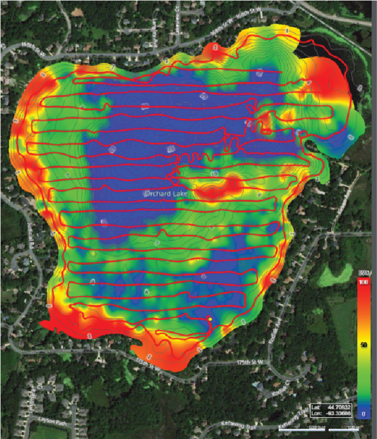
Aquatic vegetation mapping along transects

When you choose to collect aquatic plant biovolume data along predetermined transects, the resulting vegetation biovolume heat map is visually informative but based mostly on extrapolation.

Ensure to use the resulting grid data with caution. Rather use the coordinate point data along the track/transect generated in the EcoSound summary reports as these are likely more robust.

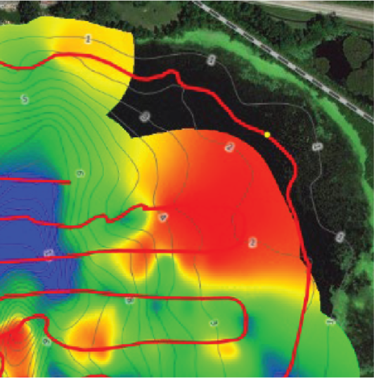
Note: The transect application is popular on large lakes where complete area coverage is not feasible or passively logging sonar/echosounder data while collecting other data (e.g. vegetation sampling).

Example of blanked output along tracks

The yellow dot on the image below is an example of a blanked output along tracks where data do not meet minimum detection requirements (too shallow).

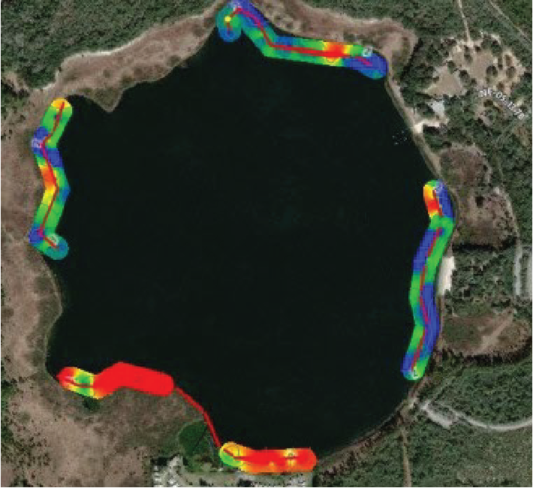
Note: In this case, the vegetation tab will not generate any report and a notification is displayed.

Example of a trip blanking

The image below is an example of a map with gaps resulting into trip blanking.

The track or map buffer can be adjusted (default is 25 m) if your tracks are spaced by more than 50 m and you want to see a complete, non-blanked map. Any increase in the buffer will also increase the grid cell size by a proportional amount such that the resultant map becomes more smoothed or generalized with increases in buffer distance.

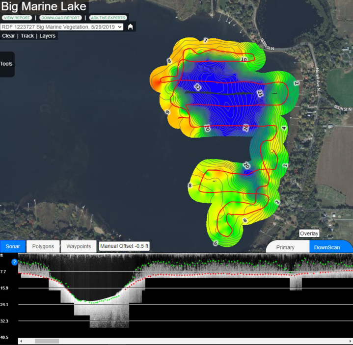
Note: Decrease the buffer where you have high transect density and would like the highest resolution possible (min is 5 m which creates 1m grid cells). This may be desirable when mapping small ponds.

Example of aquatic vegetation mapping along pre-determined transects

The biovolume heat map from these surveys is visually informative but is largely data extrapolation.

Note: Provided that there is a consistent spacing of data points along the transect, you must use point data (not grid) for your data summaries and analysis.

Full coverage aquatic vegetation mapping

Full coverage mapping in specific survey areas or whole lakes/bays is the most conventional application with EcoSound. If you need a full lake map for a very large lake, you can travel relatively fast with wide spaced transects and use a large buffer. This will give you a high-level overview of your area of interest. If you have local-scale questions, you can drive slow over narrowly spaced transects and select a narrow buffer. Both designs will generate robust grid statistics at the appropriate scale but you should exercise caution when using data collected at a coarse level to answer local scale questions (e.g., inferring invasive aquatic plant abundance in front of a property from a map with 300 m spaced transects that weren’t close to the property of interest). Contrary to transect mapping, you should generally use the grid data and statistics for analysis and summaries because data dispersion along full coverage surveys is often unbalanced and statistics could be biased. For instance, if you idled in surface growing plants while sampling aquatic plants but travelled quickly over barren areas while logging, your coverage and biovolume statistics will be biased high.